pingles

We're happy to announce the public release of a tool we've been using in production for a while now: Bifrost. 

We use Bifrost to incrementally archive all our Kafka data into Amazon S3; these transaction logs can then be ingested into our streaming data pipeline (we only need to use the archived files occasionally when we radically change our computation).

Rationale

Bifrost

Kafka is a high-throughput, persistent, distributed messaging system that was originally developed at LinkedIn. It forms the backbone of uSwitch.com’s new data analytics pipeline and this post will cover a little about Kafka and how we’re using it.

Kafka is both performant and durable. To make it easier to achieve high throughput on a single node it also does away with lots of stuff message brokers ordinarily provide (making it a simpler distributed messaging system).

Messaging

Over the past 2 years we’ve migrated from a monolithic environment based around Microsoft .NET and SQL Server to a mix of databases, applications and services. These change over time: applications and servers will come and go.

This diversity is great for productivity but has made data analytics as a whole more difficult.

We use Kafka to make it easier for the assortment of micro-applications and services, that compose to form uSwitch.com, to exchange and publish data.

Messaging helps us decouple the parts of the infrastructure letting consumers and producers evolve and grow over time with less centralised coordination or control; I’ve referred to this as building a Data Ecosystem before.

Kafka lets us consume data in realtime (so we can build reactive tools and products) and provides a unified way of getting data into long-term storage (HDFS).

Kafka’s model is pretty general; messages are published onto topics by producers, stored on disk and made available to consumers. It’s important to note that messages are pulled by consumers to avoid needing any complex throttling in the event of slow consumption.

Kafka doesn’t dictate any serialisation it just expects a payload of byte[]. We’re using Protocol Buffers for most of our topics to make it easier to evolve schemas over time. Having a repository of definitions has also made it slightly easier for teams to see what events they can publish and what they can consume.

This is what it looks like in Clojure code using clj-kafka.

We use messages to record the products that are shown across our site, the searches that people perform, emails that are sent (and bounced), web requests and more. In total it’s probably a few million messages a day.

Metadata and State

Kafka uses Zookeeper for various bits of meta-information, including tracking which messages have already been retrieved by a consumer. To that end, it is the consumers responsibility to track consumption- not the broker. Kafka’s client library already contains a Zookeeper consumer that will track the message offsets that have been consumed.

As an side, the broker keeps no state about any of the consumers directly. This keeps it simple and means that there’s no need for complex structures kept in memory reducing the need for garbage collections.

When messages are received they are written to a log file (well, handed off to the OS to write) named after the topic; these are serial append files so individual writes don’t need to block or interfere with each other.

When reading messages consumers simply access the file and read data from it. It’s possible to perform parallel consumption through partitioned topics although this isn’t something we’ve needed yet.

Messages are tracked by their offset- letting consumers access from a given point into the topic. A consumer can connect and ask for all messages that Kafka has stored currently, or from a specified offset. This relatively long retention (compared to other messaging systems) makes Kafka extremely useful to support both real-time and batch reads. Further, because it takes advantage of disk throughput it makes it a cost-effective system too.

The broker can be configured to keep messages up to a specified quantity or for a set period of time. Our broker is configured to keep messages for up to 20 days, after that and you’ll need to go elsehwere (most topics are stored on HDFS afterwards). This characteristic that has made it so useful for us- it makes getting data out of applications and servers and into other systems much easier, and more reliable, than periodically aggregating log files.

Performance

Kafka’s performance (and the design that achieves it) is derived from the observation that disk throughput has outpaced latency; it writes and reads sequentially and uses the operating system’s file system caches rather than trying to maintain its own- minimising the JVM working set, and again, avoiding garbage collections.

The plot below shows results published within an ACM article; their experiment was to measure how quickly they could read 4-byte values sequentially and randomly from different storage.

Please note the scale is logarithmic because the difference between random and sequential is so large for both SSD and spinning disks.

Interestingly, it shows that sequential disk access, spinning or SSD, is faster than random memory access. It also shows that, in their tests, sequential spinning disk performance was higher than SSD.

In short, using sequential reads lets Kafka get performance close to random memory access. And, by keeping very little in the way of metadata, the broker can be extremely lightweight.

If anyone is interested, the Kafka design document is very interesting and accessible.

Batch Load into HDFS

As I mentioned earlier, most topics are stored on HDFS so that we can maximise the amount of analysis we can perform over time.

We use a Hadoop job that is derived from the code included within the Kafka distribution.

The process looks a little like this:

Each topic has a directory on HDFS that contains 2 further subtrees: these contain offset token files and data files. The input to the Hadoop job is an offset token file which contains the details of the broker to consume from, the message offset to read from, and the name of the topic. Although it’s a SequenceFile the value bytes contain a string that looks like this:

broker.host.com topic-name  102991

The job uses a RecordReader that connects to the Kafka broker and passes the message payload directly through to the mapper. Most of the time the mapper will just write the whole message bytes directly out which is then written using Hadoop’s SequenceFileOutputFormat (so we can compress and split the data for higher-volume topics) and Hadoop’s MultipleOutputs so we can write out 2 files- the data file and a newly updated offset token file.

For example, if we run the job and consume from offset 102991 to offset 918280, this will be written to the offset token file:

broker.host.com topic-name  918280

Note that the contents of the file is exactly the same as before just with the offset updated. All the state necessary to perform incremental loads is managed by the offset token files.

This ensures that the next time the job runs we can incrementally load only the new messages. If we introduce a bug into the Hadoop load job we can just delete one or more of the token files to cause the job to load from further back in time.

Again, Kafka’s inherent persistence makes dealing with these kinds of HDFS loads much easier than dealing with polling for logs. Previously we’d used other databases to store metadata about the daily rotated logs we’d pulled but there was lots of additional computation in splitting apart files that would span days- incremental loads with Kafka are infinitely cleaner and efficient.

Kafka has helped us both simplify our data collection infrastructure, letting us evolve and grow it more flexibly, and provided the basis for building real-time systems. It’s extremely simple and very easy to setup and configure, I’d highly recommend it for anyone playing in a similar space.

Related Stuff

As I publish this LinkedIn have just announced the release of Camus: their Kafka to HDFS pipeline. The pipeline I’ve described above was inspired by the early Hadoop support within Kafka but has since evolved into something specific for use at uSwitch.

Twitter also just published about their use of Kafka and Storm to provide real-time search.

I can also recommend reading “The Unified Logging Infrastructure for Data Analytics at Twitter” paper that was published late last year.

Finally, this post was based on a brief presentation I gave internally in May last year: Kafka a Little Introduction

.

As I mentioned in an earlier article, Paul and I have produced a library to help connect Cascading and Neo4j making it easy to sink data from Hadoop with Cascading flows into a Neo4j instance. Whilst we were waiting for our jobs to run we had a little fun with some regression analysis to optimise the performance. This post covers how we did it with R.

I’m posting because it wasn’t something I’d done before and it turned out to be pretty good fun. We played with it for a day and haven’t done much else with it since so I’m also publishing in case it’s useful for others.

We improved the write performance of our library by adding support for batching- collecting mutations into sets of transactions that are batched through Neo4j’s REST API. This improved performance (rather than using a request/response for every mutation) but also meant we needed to specify a chunk size; writing all mutations in a single transaction would be impossible.

There are 2 indepent variables that we could affect to tweak performance: the batch size and the number of simultaneous connections that are making those batch calls. N.B this assumes any other hidden factors remain constant.

For us, running this on a Hadoop cluster, these 2 variables determine the batch size in combination with the number of Hadoop’s reduce or map tasks concurrently executing.

We took some measurements during a few runs of the connector across our production data to help understand whether we were making the library faster. We then produced a regression model from the data and use the optimize function to help identify the sweet spot for our job’s performance.

We had 7 runs on our production Hadoop cluster. We let the reduce tasks (where the Neo4j write operations were occurring) run across genuine data for 5 minutes and measured how many nodes were successfully added to our Neo4j server. Although the cluster was under capacity (so the time wouldn’t include any idling/waiting) our Neo4j server instance runs on some internal virtualised infrastructure and so could have exhibited variance beyond our changes.

The results for our 7 observerations are in the table below:

Regression in R

A regression lets us attempt to predict the value of a continuous variable based upon the value of one or more other independent variables. It also lets us quantify the strength of the relationship between the dependent variable and independent variables.

Given our experiment, we could determine whether batch size and the number of reducers (the independent variables) affected the number of Neo4j nodes we could create per minute (the dependent variable). If there was, we would use values for those 2 variables to predict performance.

The first stage is to load the experiment data into R and get it into a data frame. Once we’ve loaded it we can use R’s lm function to fit a linear model and look at our data.

In the above, the formula parameter to lm lets us describe that nodes.per.minute is our dependent variable (our outcome), and reducers and batch.size are our independent variables (our predictors).

Much like other analysis in R, the first thing we can look at is a summary of this model, which produces the following:

lm(formula = nodes.per.minute ~ reducers + batch.size, data = results)

Residuals:
    1     2     3     4     5     6     7 
-2330  2591 -1756 -1135  3062 -1621  1188 

Coefficients:
            Estimate Std. Error t value Pr(>|t|)  
(Intercept)   2242.8     3296.7   0.680   0.5336  
reducers       998.1      235.6   4.236   0.0133 *
batch.size     439.3      199.3   2.204   0.0922 .
---
Signif. codes:  0 ‘***’ 0.001 ‘**’ 0.01 ‘*’ 0.05 ‘.’ 0.1 ‘ ’ 1 

Residual standard error: 2735 on 4 degrees of freedom
Multiple R-squared: 0.8362, Adjusted R-squared: 0.7543 
F-statistic: 10.21 on 2 and 4 DF,  p-value: 0.02683

The summary data tells us that the model supports the data relatively well. Our R-squared is 0.075 and both batch size and reducer size are considered significant.

But, what if we tweak our model? We suspect that the shape of the performance through increasing reducers and batch size is unlikely to exhibit linear growth. We can change the formula of our model and see whether we can improve the accuracy of our model:

And let’s the the results of calling summary(model):

Call:
lm(formula = nodes.per.minute ~ reducers + I(reducers^2) + batch.size + 
    I(batch.size^2), data = results)

Residuals:
         1          2          3          4          5          6          7 
-2.433e+02  9.318e+02 -3.995e+02  9.663e-13 -7.417e+02  5.323e+01  3.995e+02 

Coefficients:
                 Estimate Std. Error t value Pr(>|t|)  
(Intercept)     -15672.16    3821.48  -4.101   0.0546 .
reducers          2755.10     337.07   8.174   0.0146 *
I(reducers^2)     -101.74      18.95  -5.370   0.0330 *
batch.size        2716.07     540.07   5.029   0.0373 *
I(batch.size^2)    -85.94      19.91  -4.316   0.0497 *
---
Signif. codes:  0 ‘***’ 0.001 ‘**’ 0.01 ‘*’ 0.05 ‘.’ 0.1 ‘ ’ 1 

Residual standard error: 948.6 on 2 degrees of freedom
Multiple R-squared: 0.9901, Adjusted R-squared: 0.9704 
F-statistic: 50.25 on 4 and 2 DF,  p-value: 0.01961

Our R-squared is now 0.9704- our second model fits the data better than our first model.

Optimization

Given the above, we’d like to understand the values for batch size and number of reducers that will give us the highest throughput.

R has an optimize function that, given a range of values for a function parameter, returns the optimal argument for the return value.

We can create a function that calls predict.lm with our model to predict values. We can then use the optimize function to find our optimal solution:

We use a set batch size of 20 and optimize to discover that the optimal number of reducers is 13 with a throughput of 22,924 nodes/minute. The second command optimizes for batch size with a fixed number of reducers. Again, it suggests a batch size of 15 for an overall throughput of 24,409 nodes/minute.

This supports what we observed earlier with the summary data: number of reducers is more significant than batch size for predicting throughput.

I’m extremely new to most of R (and statistics too if I’m honest- the last year is the most I’ve done since university) so if anyone could tell me if there’s a way to perform an optimization for both variables that would be awesome.

Please note this post was more about our experimentation and the process- I suspect our data might be prone to systematic error and problems because we only have a few observations. I’d love to run more experiments and get more measurements but we moved on to a new problem :)

Recently, I worked with a colleague (Paul Lam, aka @Quantisan on building a connector library to let Cascading interoperate with Neo4j: cascading.neo4j. Paul had been experimenting with Neo4j and Cypher to explore our data through graphs and we wanted an easy way to flow our existing data on Hadoop into Neo4j.

The data processing pipeline we’ve been growing at uSwitch.com is built around Cascalog, Hive, Hadoop and Kafka.

Once the data has been aggregated and stored a lot of our ETL is performed upon Cascalog and, by extension, Cascading. Querying/analysis is a mix of Cascalog and Hive. This layer is built upon our long-term data storage system: Hadoop; this, all combined, lets us store high-resolution data immutably at a much lower cost than uSwitch’s previous platform.

Cascading is:

application framework for Java developers to quickly and easily develop robust Data Analytics and Data Management applications on Apache Hadoop

Cascading provides a model on top of Hadoop’s very file-oriented, raw MapReduce API. It models the world around flows of data (Tuples), between Taps and according to Schemes.

For example, in Hadoop you might configure a job that reads data from a SequenceFile at a given location on HDFS. Cascading separates the 2 into slightly different concerns- the Tap would represent file storage on HDFS, the Scheme would be configured to read data according to the SequenceFile format.

Cascading provides a lot of classes to make it easier to build flows that join and aggregate data without you needing to write lots of boiler-plate MapReduce code.

Here’s an example of writing a Cascading flow (taken from the README of our cascading.neo4j library). It reads data from a delimited file (representing the Neo4j Nodes we want to create), and flows every record to our Neo4j Tap.

Although we use Cascading, really the majority of that is through Cascalog- a Clojure library that provides a datalog like language for analysing our data.

We wrote a small test flow we could use whilst testing our connector, a similar Cascalog example for the Cascading code above looks like this:

Our library, cascading.neo4j (hosted on Conjars.org) provides a Tap and Scheme suitable for sinking (writing data) to a Neo4j server using their REST connector. We extend and implement Cascading classes and interfaces making it easy to then integrate into our Cascalog processing.

cascading.neo4j allows you to create nodes, set properties on those node, add nodes to an exact match index, and create relationships (again with properties) between those nodes.

I should point out that cascading.neo4j may not be suitable for all batch processing purposes: most significantly, its pretty slow. Our production Neo4j server (on our internal virtualised infrastructure) lets us sink around 20,000 nodes per minute through the REST api. This is certainly a lot slower than Neo4j’s Batch Insert API and may make it unusable in some situations.

However, if the connector is fast enough for you it means you can sink data directly to Neo4j from your existing Cascading flows.

Performance

Whilst tweaking and tuning the connector we ran through Neo4j’s Linux Performance Guide (a great piece of technical documentation) that helped us boost performance a fair bit.

We also noticed the REST library allows for transactions to hold batch operations- to include multiple mutations in the same roundtrip. Our Neo4j RecordWriter will chunk batches- rather than writing all records in one go, you can specify the size.

We ran some tests and, on our infrastructure, using batch sizes of around 15 and 13 reducers (that is 13 ‘connections’ to our Neo4j REST api) yield the best performance of around 20,000 nodes per minute. We collected some numbers and Paul suggested we could have some fun putting those through a regression which will be the subject of my next post :)

Next steps

It’s currently still evolving a little and there’s a bit of duplicate code between the Hadoop and Local sections of the code. The biggest restrictions are it currently only supports sinking (writing) data and it’s speed may make it unsuitable for flowing very large graphs.

Hopefully this will be useful for some people and Paul and I would love pull requests for our little project.

I’m very happy to announce a very early cut of a node.js library for accessing Hadoop’s filesystem: node-hdfs. This is down to a lot of work from a colleague of mine: Horaci Cuevas.

A few months ago I was tinkering with the idea of building a Syslog to HDFS bridge: I wanted an easy way to forward web log (and other interesting data) straight out to HDFS. Given I’d not done much with node.js I thought it might be a fun exercise.

During about a week of very late nights and early mornings I followed CloudKick’s example to wrap Hadoop’s libhdfs and got as far as it reading and writing files. Horaci has picked the ball up and run far and wide with it.

After you’ve run node-waf configure && node-waf build you can write directly to HDFS:

There’s some more information in the project’s README.

Once again, massive thanks to Horaci for putting so much into the library; forks and patches most certainly welcome, I’m pretty sure the v8 C++ I wrote is wrong somehow!

We’ve been using Hadoop and Hive at Forward for just over a year now. We have lots of batch jobs written in Ruby (using our Mandy library) and a couple in Clojure (using my fork of cascading-clojure). This post covers a little of how things hang together following a discussion on the Hive mailing list around opening multiple connections to the Hive service.

Hive has some internal thread safety problems (see HIVE-80) that meant we had to do something a little boutique with HAProxy given our usage. This article covers a little about how Hive fits into some of our batch and ad-hoc processing and how we put it under HAProxy.

Background

Hive is used for both programmatic jobs and interactively by analysts. Interactive queries come via a web-based product, called CardWall, that was built for our search agency. In both cases, behind the scenes, we have another application that handles scheduling jobs, retrying when things fail (and alerting if it’s unlikely to work thereafter).

Internally, this is how things (roughly) look:

The Scheduler is responsible for knowing which jobs need to run and queuing work items. Within the batch processing application an Agent will pick up an item and check whether it’s dependencies are available (we use this to integrate with all kinds of other reporting systems, FTP sites etc.). If things aren’t ready it will place the item back on the queue with a delay (we use Beanstalkd which makes this all very easy).

Enter Hive

You’ll notice from the first screenshot we have some Hive jobs that are queued. When we first started using Hive we started using a single instance of the HiveServer service started as follows: $HIVE_HOME/bin/hive --service hiveserver. Mostly this was using a Ruby Gem called RBHive.

This worked fine when we were using it with a single connection, but, we ran into trouble when writing apps that would connect to Hive as part of our batch processing system.

Originally there was no job affinity, workers would pick up any piece of work and attempt it, and with nearly 20 workers this could heavily load the Hive server. Over time we introduced different queues to handle different jobs, allowing us to allocate a chunk of agents to sensitive resources (like Hive connections).

Multiple Hive Servers

We have a couple of machines that run multiple HiveServer instances. We use Upstart to manage these processes (so have hive1.conf, hive2.conf… in our /etc/init directory). Each config file specifies a port to open the service on (10001 in the example below).

These are then load-balanced with HAProxy, the config file we use for that is below

It was Forward's first hackday last Friday. Tom Hall and I worked on some collaborative filtering using Mahout and Hadoop to process some data collected from Twitter.

I'd been collecting statuses through their streaming API (using some code from a project called Twidoop). After wrestling with formats for a little while we realised that each JSON record was separated by a null character (all bits zeroed). There didn't seem to be an easy way to change the terminating character for the TextInputFormat that we'd normally use so we wrote our own InputFormat and I'm posting it here for future reference (and anyone else looking for a Hadoop InputFormat to process similar files).

We added it to my fork of cascading-clojure but it will work in isolation.

This is something that I’ve been battling with for a while and tonight, whilst not able to sleep, I finally found a way to crack it! The answer: use an XmlInputFormat from a related project. Now for the story.

We process lots of XML documents every day and some of them are pretty large: over 8 gigabytes uncompressed. Each. Yikes!

We’d made significant performance gains by switching the old REXML SAX parser to libxml. But we’ve suffered from random segfaults on our production servers (seemingly caused by garbage collecting bad objects). Besides, this still was running at nearly an hour for the largest reports.

Hadoop did seem to offer XML processing: the general advice was to use Hadoops’s StreamXmlRecordReader which can be accessed through using the StreamInputFormat.

This seemed to have weird behaviour with our reports (which often don’t have line-endings): lines would be duplicated and processing would jump to 100%+ complete. All a little fishy.

Hadoop Input Formats and Record Readers

The InputFormat in Hadoop does a couple of things. Most significantly, it provides the Splits that form the chunks that are sent to discrete Mappers.

Splits form the rough boundary of the data to be processed by an individual Mapper. The FileInputFormat (and it’s subclasses) generate splits on overall file size. Of course, it’s unlikely that all individual Records (a Key and Value that are passed to each Map invocation) lie neatly within these splits: records will often cross splits. The RecordReader, therefore, must handle this

… on whom lies the responsibilty to respect record-boundaries and present a record-oriented view of the logical InputSplit to the individual task.

In short, a RecordReader could scan from the start of a split for the start of it’s record. It may then continue to read past the end of it’s split to find the end. The InputSplit only contains details about the offsets from the underlying file: data is still accessed through the streams.

It seemed like the StreamXmlRecordReader was skipping around the underlying InputStream too much; reading records it wasn’t entitled to read. I tried my best at trying to understand the code but it was written a long while ago and is pretty cryptic to my limited brain.

I started trying to rewrite the code from scratch but it became pretty hairy very quickly. Take a look at the implementation of next() in LineRecordReader to see what I mean.

Mahout to the Rescue

After a little searching around on GitHub I found another XmlInputFormat courtesy of the Lucene sub-project: Mahout.

I’m happy to say it appears to work. I’ve just run a quick test on our 30 node cluster (via my VPN) and it processed the 8 gig file in about 10 minutes. Not bad.

For anyone trying to process XML with Hadoop: try Mahout’s XmlInputFormat.

The quantity of data we analyse at Forward every day has grown nearly ten-fold in just over 18 months. Today we run almost all of our automated daily processing on Hadoop. The vast majority of that analysis is automated using Ruby and our open-source gem: Mandy.

In this post I’d like to cover a little background to MapReduce and Hadoop and a light introduction to writing a word count in Ruby with Mandy that can run on Hadoop.

Mandy’s aim is to make MapReduce with Hadoop as easy as possible: providing a simple structure for writing code, and commands that make it easier to run Hadoop jobs.

Since I left ThoughtWorks and joined Forward in 2008 I’ve spent most of my time working on the internal systems we use to work with our clients, track our ads, and analyse data. Data has become truly fundamental to our business.

I think it’s worth putting the volume of our processing in numbers: we track around 9 million clicks a day across our campaigns- averaged out across a day that’s over 100 every second (it actually peaks up to around 1400 a second).

We automate the analysis, storage, and processing of around 80GB (and growing) of data every day. In addition, further ad-hoc analysis is performed through the use of a related project: Hive (more on this in a later blog post).

We’d be hard pressed to work with this volume of data in a reasonable fashion, or be able to change what analysis we run, so quickly if it wasn’t for Hadoop and it’s associated projects.

Hadoop is an open-source Apache project that provides “open-source software for reliable, scalable, distributed computing”. It’s written in Java and, although relatively easy to get into, still falls foul of Java development cycle problems: they’re just too long. My colleague (Andy Kent) started writing something we could prototype our jobs in Ruby quickly, and then re-implement in Java once we understood things better. However, this quickly turned into our platform of choice.

To give a taster of where we’re going, here’s the code needed to run a distributed word count:

And how to run it?

mandy-hadoop wordcount.rb hdfs-dir/war-and-peace.txt hdfs-dir/wordcount-output

The above example comes from a lab Andy and I ran a few months ago at our office. All code (and some readmes) are available on GitHub.

What is Hadoop?

The Apache Hadoop project actually contains a number of sub-projects. MapReduce probably represents the core- a framework that provides a simple distributed processing model, which when combined with HDFS provides a great way to distribute work across a cluster of hardware. Of course, it goes without saying that it is very closely based upon the Google paper.

Parallelising Problems

Google’s MapReduce paper explains how, by adopting a functional style, programs can be automatically parallelised across a large cluster of machines. The programming model is simple to grasp and, although it takes a little getting used to, can be used to express problems that are seemingly difficult to parallelise.

Significantly, working with larger data sets (both storage and processing) can be solved by growing the cluster’s capacity. In the last 6 months we’ve grown our cluster from 3 ex-development machines to 25 nodes and taken our HDFS storage from just over 1TB to nearly 40TB.

An Example

Consider an example: perform a subtraction across two sets of items. That is

{1,2,3} - {1,2} = {3}

. A naive implementation might compare every item for the first set against those in the second set.

numbers = [1,2,3]
[1,2].each { |n| numbers.delete(n) }

This is likely to be problematic when we get to large sets as the time taken will grow very fast (m*n). Given an initial set of 10,000,000 items, finding the distinct items from a second site of even 1,000 items would result in 10 billion operations.

However, because of the way the data flows through a MapReduce process, the data can be partitioned across a number of machines such that each machine performs a smaller subset of operations with the result then combined to produce a final output.

It’s this flow that makes it possible to ‘re-phrase’ our solution to the problem above and have it operate across a distributed cluster of machines.

Overall Data Flow

The Google paper and a Wikipedia article provide more detail on how things fit together, but here’s the rough flow.

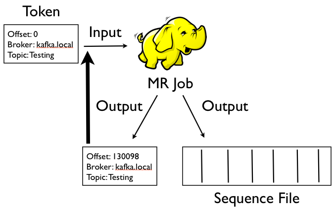
Map and reduce functions are combined into one or more ‘Jobs’ (almost all of our analysis is performed by jobs that pass their output to further jobs). The general flow can be seen to be made of the following steps:

1. Input data read
2. Data is split
3. Map function called for each record
4. Shuffle/sort
5. Sorted data is merged
6. Reduce function called
7. Output (for each reducer) written to a split
8. Your application works on a join of the splits

First, the input data is read and partitioned into splits that are processed by the Map function. Each map function then receives a whole ‘record’. For text files, these records will be a whole line (marked by a carriage return/line feed at the end).

Output from the Map function is written behind-the-scenes and a shuffle/sort performed. This prepares the data for the reduce phase (which needs all values for the same key to be processed together). Once the data has been sorted and distributed to all the reducers it is then merged to produce the final input to the reduce.

Map

The first function that must be implemented is the map function. This takes a series of key/value pairs, and can emit zero or more pairs of key/value outputs. Ruby already provides a method that works similarly: Enumerable#map.

For example:

names = %w(Paul George Andy Mike)
names.map {|name| {name.size => name}} # => [{4=>"Paul"}, {6=>"George"}, {4=>"Andy"}, {4=>"Mike"}]

The map above calculates the length of each of the names, and emits a list of key/value pairs (the length and names). C# has a similar method in ConvertAll that I mentioned in a previous blog post.

Reduce

The reduce function is called once for each unique key across the output from the map phase. It also produces zero or more key value pairs.

For example, let’s say we wanted to find the frequency of all word lengths, our reduce function would look a little like this:

def reduce(key, values)
  {key => values.size}
end

Behind the scenes, the output from each invocation would be folded together to produce a final output.

To explore more about how the whole process combines to produce an output let’s now turn to writing some code.

Code: Word Count in Mandy

As I’ve mentioned previously we use Ruby and Mandy to run most of our automated analysis. This is an open-source Gem we’ve published which wraps some of the common Hadoop command-line tools, and provides some infrastructure to make it easier to write MapReduce jobs.

Installing Mandy

The code is hosted on GitHub, but you can just as easily install it from Gem Cutter using the following:

$ sudo gem install gemcutter
$ gem tumble
$ sudo gem install mandy

… or

$ sudo gem install mandy --source http://gemcutter.org

If you run the mandy command you may now see:

You need to set the HADOOP_HOME environment variable to point to your hadoop install    :(
Try setting 'export HADOOP_HOME=/my/hadoop/path' in your ~/.profile maybe?

You’ll need to make sure you have a 0.20.x install of Hadoop, with HADOOP_HOME set and $HADOOP_HOME/bin in your path. Once that’s done, run the command again and you should see:

You are running Mandy!
========================

Using Hadoop 0.20.1 located at /Users/pingles/Tools/hadoop-0.20.1

Available Mandy Commands
------------------------
mandy-map       Run a map task reading on STDIN and writing to STDOUT
mandy-local     Run a Map/Reduce task locally without requiring hadoop
mandy-rm        remove a file or directory from HDFS
mandy-hadoop    Run a Map/Reduce task on hadoop using the provided cluster config
mandy-install   Installs the Mandy Rubygem on several hosts via ssh.
mandy-reduce    Run a reduce task reading on STDIN and writing to STDOUT
mandy-put       upload a file into HDFS

If you do, you’re all set.

Writing a MapReduce Job

As you may have seen earlier to write a Mandy job you can start off with as little as:

Of course, you may be interested in writing some tests for your functions too. Well, you can do that quite easily with the Mandy::TestRunner. Our first test for the Word Count mapper might be as follows:

Our implementation for this might look as follows:

Of course, our real mapper needs to do more than just tokenise the string. It also needs to make sure we downcase and remove any other characters that we want to ignore (numbers, grammatical marks etc.). The extra specs for these are in the mandy-lab GitHub repository but are relatively straightforward to understand.

Remember that each map works on a single line of text. We emit a value of 1 for each word we find which will then be shuffled/sorted and partitioned by the Hadoop machinery so that a subset of data is sent to each reducer. Each reducer will, however, receive all the values for that key. All we need to do in our reducer is sum all the values (all the 1’s) and we’ll have a count. First, our spec:

And our implementation:

In fact, Mandy has a number of built-in reducers that can be used (so you don’t need to re-implement this). To re-use the Sum-ming reducer replace the reduce statement above to reduce(Mandy::Reducers::SumReducer).

Our mandy-lab repository includes some sample text files you can run the examples on. Assuming you’re in the root of the repo you can then run the following to perform the wordcount across Alice in Wonderland locally:

$ mandy-local word_count.rb input/alice.txt output
Running Word Count...
/Users/pingles/.../output/1-word-count

If you open the /Users/pingles/.../output/1-word-count file you should see a list of words and their frequency across the document set.

Running the Job on a Cluster

The mandy-local command just uses some shell commands to imitate the MapReduce process. If you try running the same command over a larger dataset you’ll come unstuck. So let’s see how we run the same example on a real Hadoop cluster. Note, that for this to work you’ll need to either have a Hadoop cluster or Hadoop running locally in pseudo-distributed mode.

If you have a cluster up and running, you’ll need to write a small XML configuration file to provide the HDFS and JobTracker connection info. By default the mandy-hadoop command will look for a file called cluster.xml in your working directory. It should look a little like this:

<?xml version="1.0" encoding="UTF-8"?>
<configuration>
  <property>
    <name>fs.default.name</name>
    <value>hdfs://datanode:9000/</value>
  </property>
  <property>
    <name>mapred.job.tracker</name>
    <value>jobtracker:9001</value>
  </property>
  <property>
    <name>hadoop.job.ugi</name>
    <value>user,supergroup</value>
  </property>
</configuration>

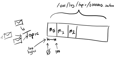
Once that’s saved, you need to copy your text file to HDFS so that it can be distributed across the cluster ready for processing. As an aside: HDFS shards data in 64MB blocks across the nodes. This provides redundancy to help mitigate in the case of machine failure. It also means the job tracker (the node which orchestrates the processing) can move the computation close to the data and avoid copying large amounts of data unnecessarily.

To copy a file up to HDFS, you can run the following command

$ mandy-put my-local-file.txt word-count-example/remote-file.txt

You’re now ready to run your processing on the cluster. To re-run the same word count code on a real Hadoop cluster, you change the mandy-local command to mandy-hadoop as follows:

$ mandy-hadoop word_count.rb word-count-example/remote-file.txt word-count-example/output

Once that’s run you should see some output from Hadoop telling you the job has started, and where you can track it’s progress (via the HTTP web console):

Packaging code for distribution...
Loading Mandy scripts...

Submitting Job: [1] Word Count...
Job ID: job_200912291552_2336
Kill Command: mandy-kill job_200912291552_2336 -c /Users/pingles/.../cluster.xml
Tracking URL: http://jobtracker:50030/jobdetails.jsp?jobid=job_200912291552_2336

word-count-example/output/1-word-count

Cleaning up...
Completed Successfully!

If you now take a look inside ./word-count-example/output/1-word-count you should see a few part-xxx files. These contain the output from each reducer. Here’s the output from a reducer that ran during my job (running across War and Peace):

abandoned   54
abandoning  26
abandonment 14
abandons    1
abate   2
abbes   1
abdomens    2
abduction   3
able    107

Wrap-up

That’s about as much as I can cover in an introductory post for Mandy and Hadoop. I’ll try and follow this up with a few more to show how you can pass parameters from the command-line to Mandy jobs, how to serialise data between jobs, and how to tackle jobs in a map and reduce stylee.

As always, please feel free to email me or comment if you have any questions, or (even better) anything you’d like me to cover in a future post.